As my previous blog post  concluded we had decided upon a selection of algorithms to try out. These were:

1. Trees
2. Lazy (kNN)
3. Neural Networks
4. Voting

Choosing good flags

Flags are treated independently, like in MILEPOST. Due to this, determining what merits a ‘good’ flag that shows some effect in improving the energy efficiency can be done in a simple way that sticks with the independent model. Looking at the results of 500 random flags turned on and off, along with the coinciding energy usage, means that some visual analysis can be performed.

A ratio of how often each flag appears in passes that perform better than the standard -O3 level can be determined, along with the ratio of how often that flag appears in all other solutions. Once this information is gained it can be used to see if there is a clear existence of a flag appearing consistently more frequently in better passes, and therefore having some link to performing better. An example of this is given below:

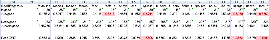
In this example, there are 43 passes from the 500 run that performed better than standard -O3. From this we can see that the column ‘In good’ determines a count of how many times each flag appears in those 43 passes. Ones that appear frequently (>60%) are marked as potential ‘good’ flags. Then for the remaining 457 passes, the same calculation can be performed. With both ratios calculated we look for flags whose good ratio is significantly higher than their not good one. This is given a numerical value by dividing the good ratio by the not good one, the higher the resulting number the better the flag. This is our indication that the flags presence is a stimulus in improvement for energy efficiency.

All data collected was from using the BEEBS framework.

Results and reliability

Trees

1. J48
   • Performs fastest of the lot
   • Accuracy from results we had was 100%
2. PART
   • Tree variant that performs slightly worse than J48 in this case
3. Ridor
   • 95.42% accuracy which was the worst of the set
   • Believed to be due to pruning
4. LADTree
   • Good results, another form of tree variant and comparable to J48

Lazy

1. KNN
   • 100% accuracy used alone

Functions

1. SMO
   • Type of SVM that kept speedy but suffered slight inaccuracy
2. Multilayer Perceptron
   • Neural networks proved to give good results, however it is a slow algorithm that is proved by taking nearly 20x time to run over 9 sets of data
   • We can see it is good but becomes a bottleneck to train with very large training sets

Voting

1. KNN + J48
   • Resulted in same accuracy of 100%
   • Good method because classifies using both algorithms and chooses majority vote or the one most likely to be true of both
2. J48 + SMO
   • Resulted in accuracy of 99.5%
3. J48 + Multilayer Perceptron
   • Accuracy of 100%
   • Very slow due to double classification using neural nets

Discussion

Despite all the high accuracy and the results provided, we cannot take this with too much reliability, simply due to the lack of data for analysis. There were 9 programs from the BEEBS framework and each run under 500 random on/off flag settings, but realistically for concrete analysis we need 100+ programs with this data available.

So, although we can gain some information such as that Multilayer Perceptron would seemingly bottleneck when we expand our data set, and that J48 seems to perform quite fast out of the lot, the results cannot be used reliably. But for now it provides insights and a direction to explore. I hope to solve this problem as I will continue this for my final year project and aim to expand this set along with its readings, as well as to then re-run all of the above algorithms and analyse the results again for some more reliable results.